US Election Principal Component Analysis

Summary: While the alliance of US states to particular parties fluctuates, regional voting blocks are much more persistent. The primary regional voting blocks are Union North vs. Confederate South and Urban East vs. Rural West.

Skip to Methodology

Data Visualizations

Maps

Principal Component 1

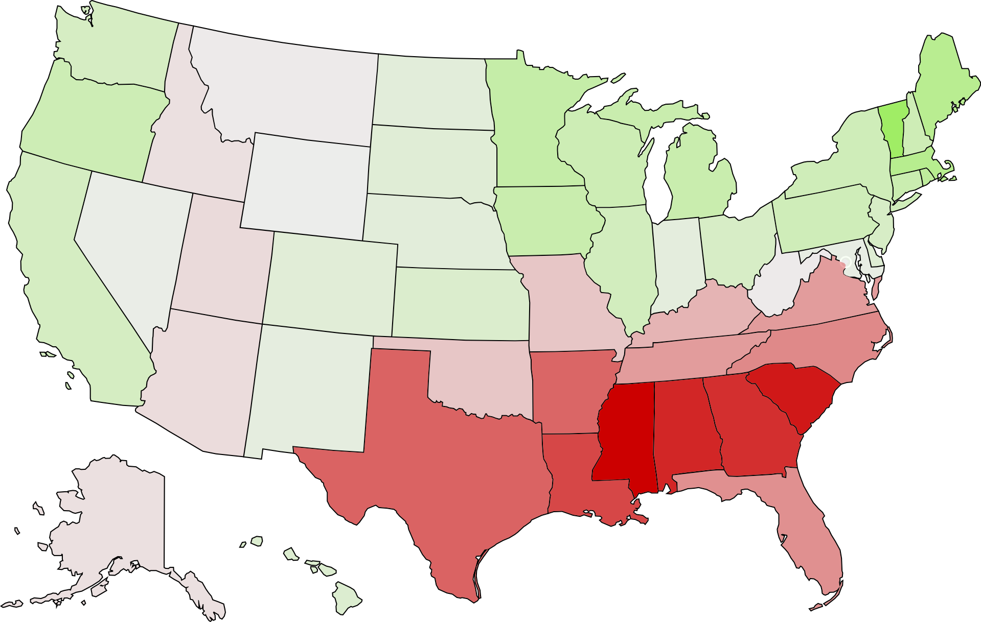
Principal Component 1 strongly correlates to North-South. Specifically, it correlates to American Civil War.

• There is a perfect correlation between the 11 states that seceded to form the Confederacy and the 11 states with the lowest PC1 scores (PC1 < -10).
• The 15 highest PC1 scores are 15 out of the 20 states that fought for the Union (PC1 > +7.0).
• The 19 states near the middle of the PC1 scale (-5.0 < PC1 < +5.0) are universally either border states which were divided during the Civil War (e.g. West Virgina, Maryland), or states that did not yet exist during the Civil War (e.g. New Mexico, Wyoming), or Indiana¹.

Principal Component 2

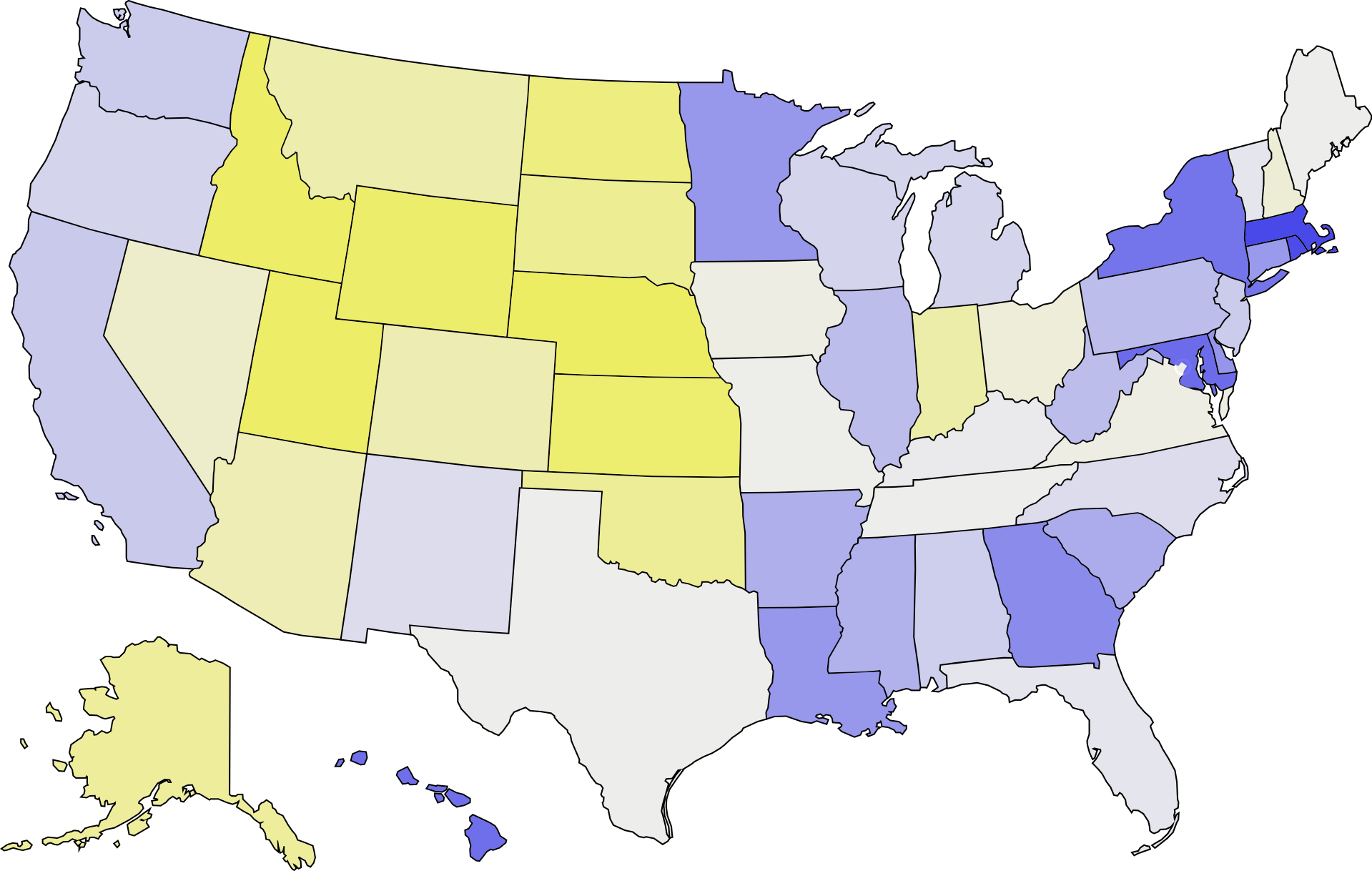
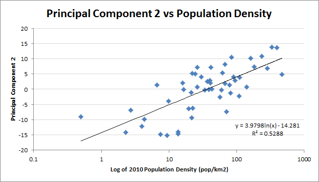
Principal Component 2 strongly correlates to Urban East vs. Rural West.

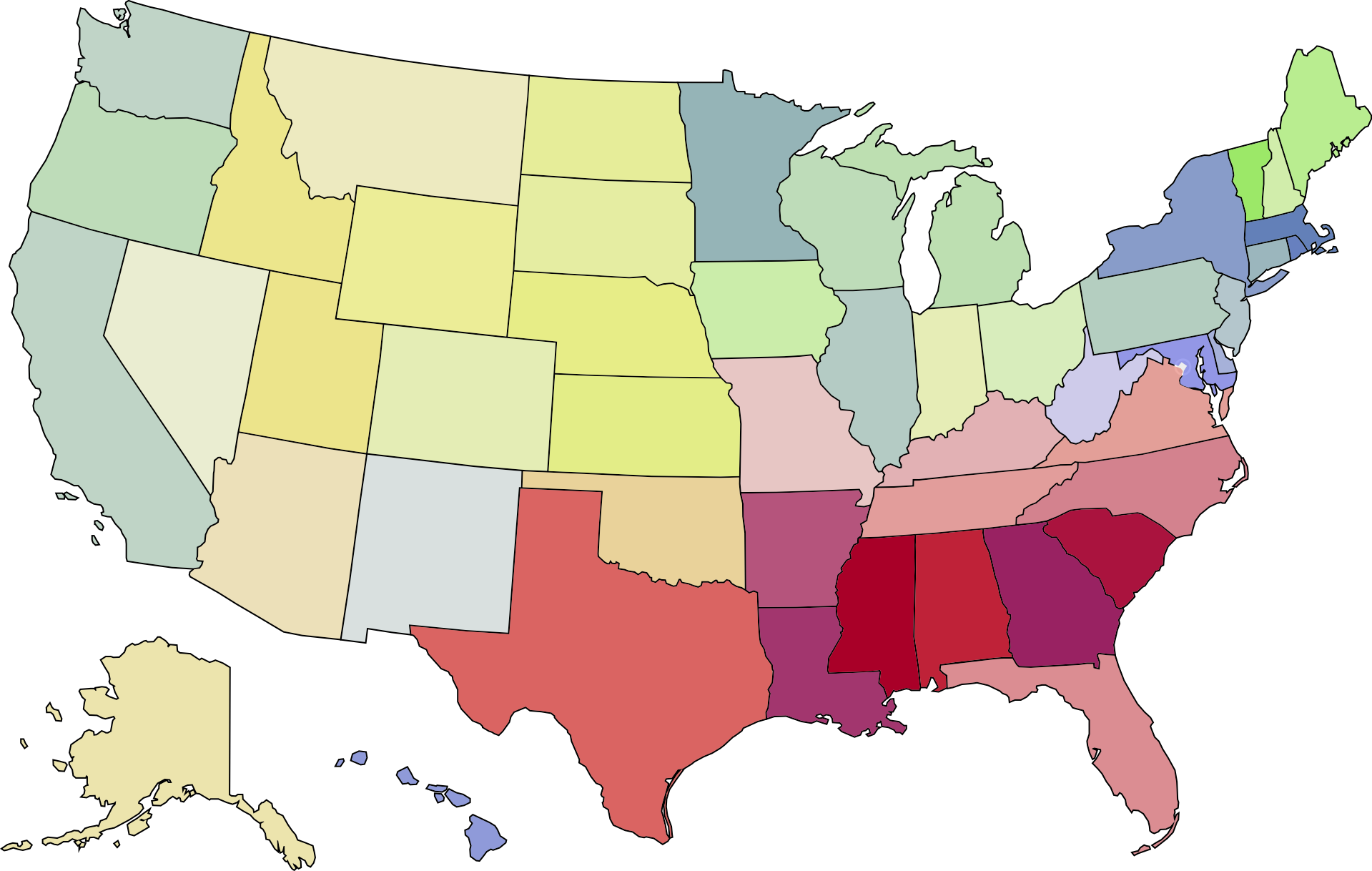
Components 1 and 2 Overlaid

State map colored by Principal Components 1 and 2 overlaid

Scatter Plot

Scatter Plot of States by first two Principal Components

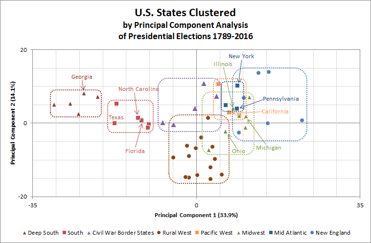
The points colored by geographical regions. All points in a region are outlined by a cluster border in the same color. The top 10 states by 2010 population are labelled.

You can see again here that New England really patterns as two clusters, which I call Greater Plymouth (Massachusetts and Rhode Island very close, with Connecticut slightly further away) and the Far North (New Hampshire, Vermont, and Maine). The Far North states are much more rural than Greater Plymouth and pattern correspondingly closer to the Rural West on PC2.

The Midwest Cluster would be much tighter without the Indiana² point that is out towards the middle of the Rural West cluster instead.

Similarly, the Rural West cluster would be noticeably tighter if New Mexico was left out, the only Rural West state on the far side of the middle point on PC2, on the edge of the Pacific West cluster.

Dendrogram

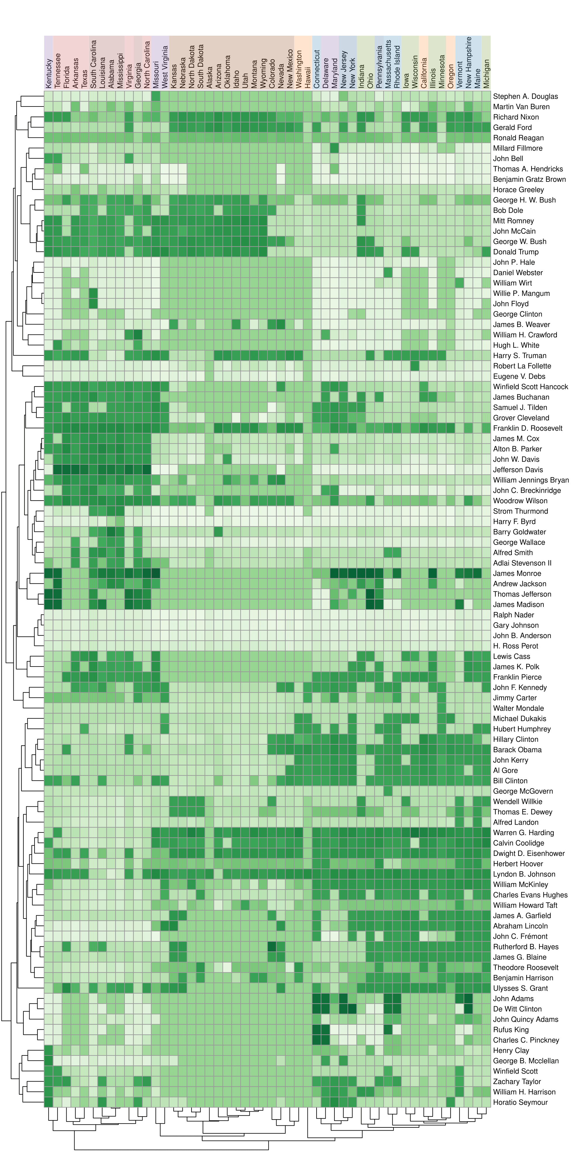
Each box is colored by overall support level for a State-Candidate pair. White means 0 support and dark green means full support from the state.

The dendrograms on the top and left show the parsimonious hierarchical clustering of states and candidates, respectively. Corresponding to the data patterns seen in other visualizations, the first two splits divide the states into South, Rural West, East/Everything Else; with the 5 Border States being distributed evenly among the three groups (1, 2, and 1, respectively).

Methodology

PCA Input Features

• Candidate Electoral Support per State-Year (159 features per state, 10 discarded for insufficient variability)
• Candidate Popular Support per State-Year (159 features per state, 40 discarded)
• Party Electoral Support per State-Year (141 features per state, 11 discarded)
• Party Popular Support per State-Year (141 features per state, 27 discarded)

Total features used: 512

I used both candidate and party support to capture situations in which a party's vote is split between multiple candidates, but two states that vote for different candidates from the same party may be more similar than states that vote for different candidates from different parties. For example, in 1836 the Whig party intentionally ran three different candidates in different regions to try to prevent Martin Van Buren from receiving a majority of electoral votes (unsuccessfully).

In many early years, no popular vote is recorded (and may not have occurred with the electors being appointed by the state legislature instead of by popular vote) so a number of the popular vote features are discarded for null data. Some portion of the remaining features were discarded as insufficiently variable, such as Martin Van Buren's electoral support in 1848, which was 0 in all states. (But his popular support feature for 1848 is retained, capturing the variation in his support state by state from 0% to 28%.)

PCA Output Components

Once I had the input features, I used the ClustVis PCA web tool to perform the analysis.

The first two components overwhelmingly dominate the data. The first component roughly corresponds to North/South opposition and accounts for 34% of the data variability. The second component roughly corresponds to East/West (or Urban/Rural) opposition and accounts for another 14% of the data variability, for a cumulative 48% of the variability captured by the first two components.

The third component accounts for about 5% of the data variability, and all other components are less than 5% of the variability each.

Regional Clusters used in Scatter Plot mapped

Border States

Civil war definition: States that allowed slavery, but that never seceded from the union.

New England

Standard definition

South and Deep South

The states that seceded during the Civil War. My distinction between these two cartegories is based on the results of my clustering, but my "Deep South" corresponds to the five states most often included in various definitions of "Deep South".

Mid Atlantic

Standard definition minus states that qualify as "Border States" or "South"

Midwest

States bordering the Great Lakes or the Mississippi River that do not qualify in any other category

Pacific West

The states touching the Pacific Ocean, minus Alaska

Rural West

All states west of the Mississippi River that do not border on the Mississippi River, the Gulf of Mexico, or the Pacific Ocean, plus Alaska.

Dendrogram

The dendrogram and its clustering are also produced by ClustVis, on a slightly different data set that compresses all of the data into a single Overall Support value for each State-Candidate pair.

Overall Support for a State-Candidate pair is calculated by combining both electoral support and popular support (where applicable). If a candidate participated in more than one election, only the average for each state across elections is used in the dendrogram.

Where no Overall Support value exists for a State-Candidate pair (usually for an elections that took place before a state joined the union), the value is interpolated to a neutral average.

This optimizes the data for clustering states, but sometimes fails to properly cluster candidates. For example, Robert La Follete and Eugene Debs should properly cluster with the rest of the third party candidates with broad but very shallow support (see the Nader-Johnson-Anderson-Perot cluster), but don't because their campaigns were before Alaska and Hawai'i voted, and the "neutral average" interpolated for Alaska and Hawai'i in this case is significantly more than the minimal support they received from other states, so the clustering algorithm incorrectly concludes La Follete and Debs form a separate cluster of Candidates who perform better in Alaska and Hawai'i than in any other state.

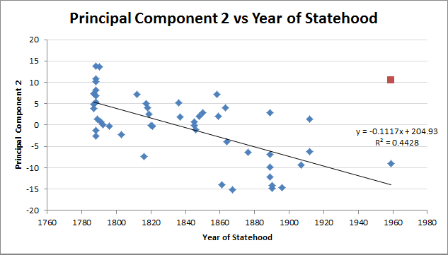
States clustering shouldn't be to distorted by this effect, though. If they were, PC2 should correlate more strongly with year of statehood (R² = 0.29) than with population density (R²=0.53), instead of vice versa.

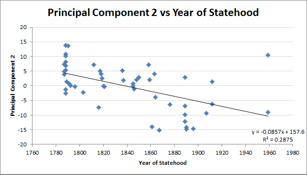
The correlation with year of statehood improves considerably if Hawai'i is discarded as an outlier (R² = 0.44), but it is still weaker than the correlation with log population density (R² = 0.53). Since year of statehood and population density are themselves correlated, the weaker of the two correlations with PC2 is being inflated by the stronger (and vice versa, but not as much).

Footnootes

• ¹²Indiana is Weird: https://fivethirtyeight.com/features/indiana-is-weird/